Processing Enzymatic Sequences via Deep Learning

1. Data Processing

a) Dataset Cleanup

After importing data as a CSV file into our notebook, we performed several treatments:

• Removal of unnecessary columns.
• Elimination of missing values (NaN), generated during Excel import.
• Column renaming for better readability.

We also filtered data by removing certain rows marked as unreliable, particularly those containing ”-” symbols in the Induction (Gel) and Expression (Gel) columns.

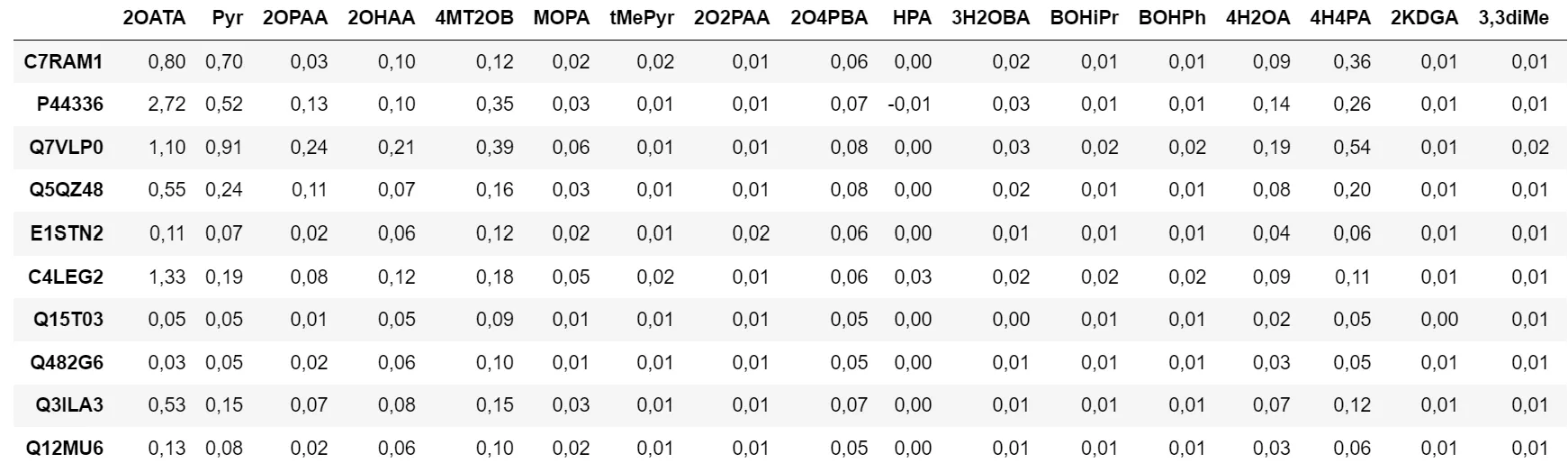
Figure 1 - Data Table

Additionally, we store certain data like Bradford and purities in dictionaries for later use in the model:

bradford = {}
for line in range(8, len(df.index)):
    bradford[df.index[line]] = float(df['Bradford (mg/mL)'][line].replace(',', '.'))

purities = {}
for row in range(len(df.columns)):
    if df[df.columns[row]]['Pureté'] !=  '---':
        purities[df.columns[row]] = int(df[df.columns[row]]['Pureté'][:-1])
    else:
        purities[df.columns[row]] = 100

b) Sequence Processing

By importing the fasta file, we add sequences to a dictionary with the common name as key and the complete sequence as object. The re module allows searching for the common name in the header line, then we start by normalizing data with the Bradford we previously recorded:

for line in range(len(df.index)):
    for row in range(len(df.columns)):
        n_line = df.index[line]
        n_row = df.columns[row]
        cell = df[n_row][n_line]
        df[n_row][n_line] = float(cell.replace(',', '.')) / bradford[n_line]

c) Sequence Alignment

For this, we used Clustal2, an executable that performs data alignment taking a Fasta file as input. For this, we use a module called ClustalwCommandline.

Figure 2 - Clustal2 Executable

clustalw_exe = "clustalw2.exe" # Location of the executable that will process them
output_file = "output.aln"
input_file = "FASTAs_Final.fasta"

sequences = list(SeqIO.parse(input_file, "fasta"))
seq_records = [SeqRecord(seq.seq, id=seq.id) for seq in sequences]
# Create a SeqRecord object for each sequence

temp_file = "temp.fasta" # Create a temporary file to store sequences
SeqIO.write(seq_records, temp_file, "fasta")

clustalw_cline = ClustalwCommandline(
# Initialize ClustalwCommandline object to properly process data
     cmd=clustalw_exe,
     infile=input_file,
     outfile=output_file,
     output="clustal",  # Output format
     align=True,  # Perform complete alignment
)

clustalw_cline()
# Execute ClustalW2 command

aligned_sequences = list(SeqIO.parse(output_file, "clustal"))
# Now we can read aligned sequences

After a processing time of about 5 minutes, we end up with aligned sequences in this form:

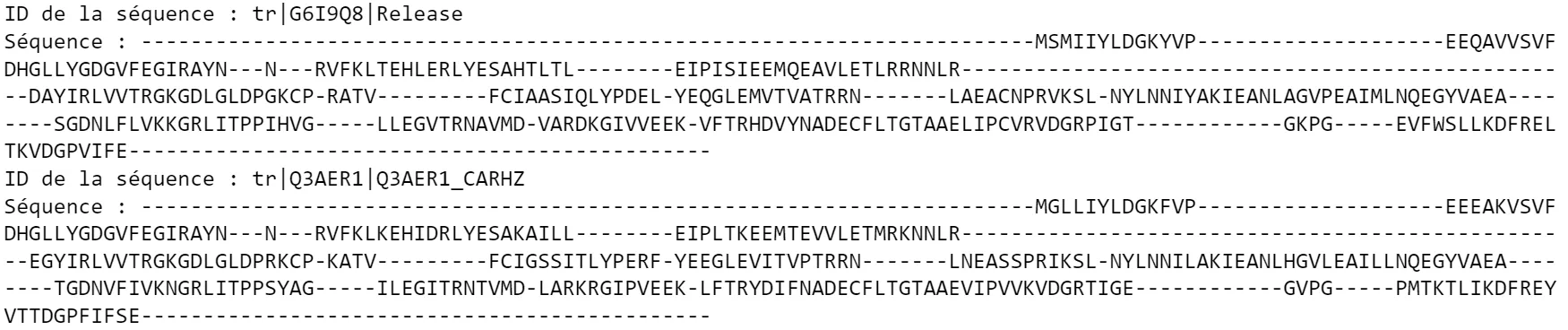
Figure 3 - Sequence Alignment Result

2. AI Models

To be able to use the sequences of different enzymes we have, we had to “encode” them to provide our neural network with numerical values.

The choice that seemed most relevant was to match each (A,B,C…) to numbers (1,2,3…) to obtain a numpy array of integers of length 546 for each sequence.

sequence = "-AB--TGA(..)ALA---"
encoded sequence = [0,1,2,0,0,(..)1,12,1,0,0,0]

For the ’-’ induced by sequence alignment, we decided to assign it the number 0.

a) First Model: Classic Dense Network

To start, we first performed initial tests with a very basic model, using only a few layers of interconnected neurons:

model = Sequential()
model.add(Dense(100, activation="relu", input_shape=(546,)))
model.add(Dense(150, activation="relu"))
model.add(Dense(50, activation="relu"))
model.add(Dense(18))

Thus, from the inputs we provide (encoded sequences as arrays), the model predicts 18 output values, corresponding to the 18 sought activities for different substrates.

We then trained this model on all sequences that we previously separated into train and test data:

X_train, X_test, y_train, y_test = train_test_split(X, y, test_size=0.2, random_state=78)

Here we obtain the train loss (blue) and test loss (yellow).

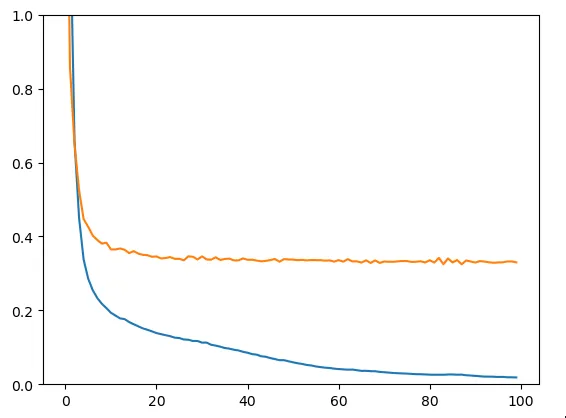
Figure 4 - Train & Test Loss

We clearly face an overfitting problem: the model learns input data by heart while failing to generalize on data it hasn’t seen during training. The model is therefore not suitable: let’s try to create a slightly more evolved one.

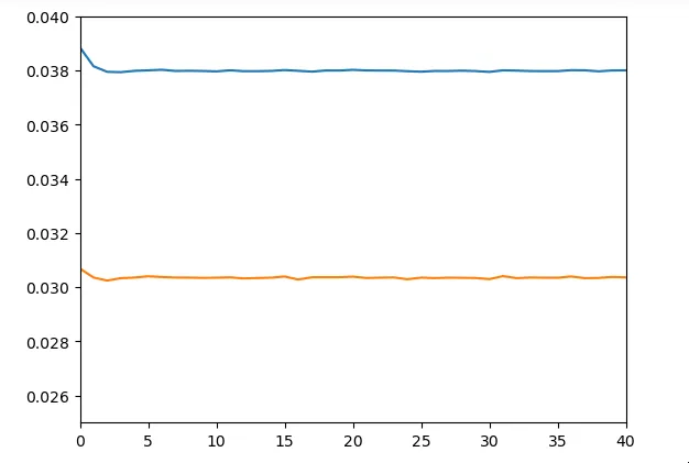
b) Second Model: Slightly More Evolved Dense Network

Here is a more performant architecture:

model = Sequential()
model.add(Dense(500, activation="relu", input_shape=(546,)))
model.add(BatchNormalization())
model.add(Dropout(0.3))
model.add(Dense(300, activation="relu"))
model.add(BatchNormalization())
model.add(Dropout(0.2))
model.add(Dense(200, activation="relu"))
model.add(BatchNormalization())
model.add(Dropout(0.3))
model.add(Dense(100, activation="relu"))
model.add(BatchNormalization())
model.add(Dense(50, activation="relu"))
model.add(Dropout(0.2))
model.add(Dense(18))

We introduced Dropout, allowing to randomly deactivate a certain percentage of neurons in each layer during training, with the objective of preventing memorization of data and favoring generalization. Additionally, to improve training stability and accelerate convergence, we added BatchNormalization layers.

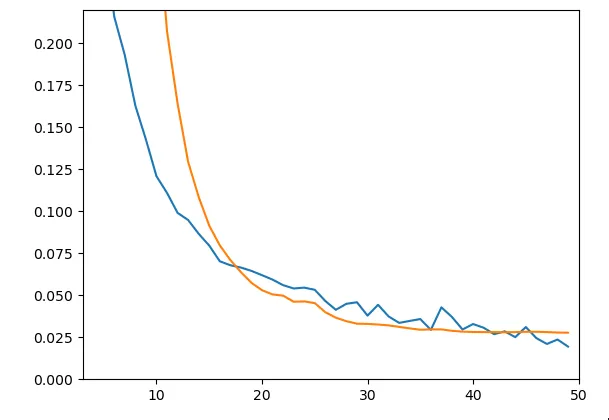
Figure 5 - Train & Test Loss

As can be seen in the graph, results are significantly better in terms of generalization ability (little gap between the two curves). We obtain a test loss of about 0.028. Yet when looking at predictions, we notice it’s not very conclusive. Here are predictions and expected values for enzyme C7RAM1, for different substrates:

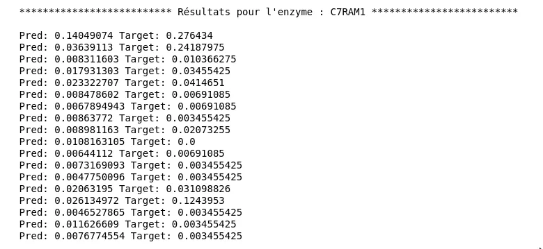
Figure 6 - Results for the Second Model

Although some predictions have the right order of magnitude, there is a non-negligible gap.

c) Third Model: 1D Convolutional Network

We therefore tried to implement a 1D convolutional network. This type of network is very interesting because it allows better spatial data processing, thanks to 1D filters that will traverse our enzyme sequences.

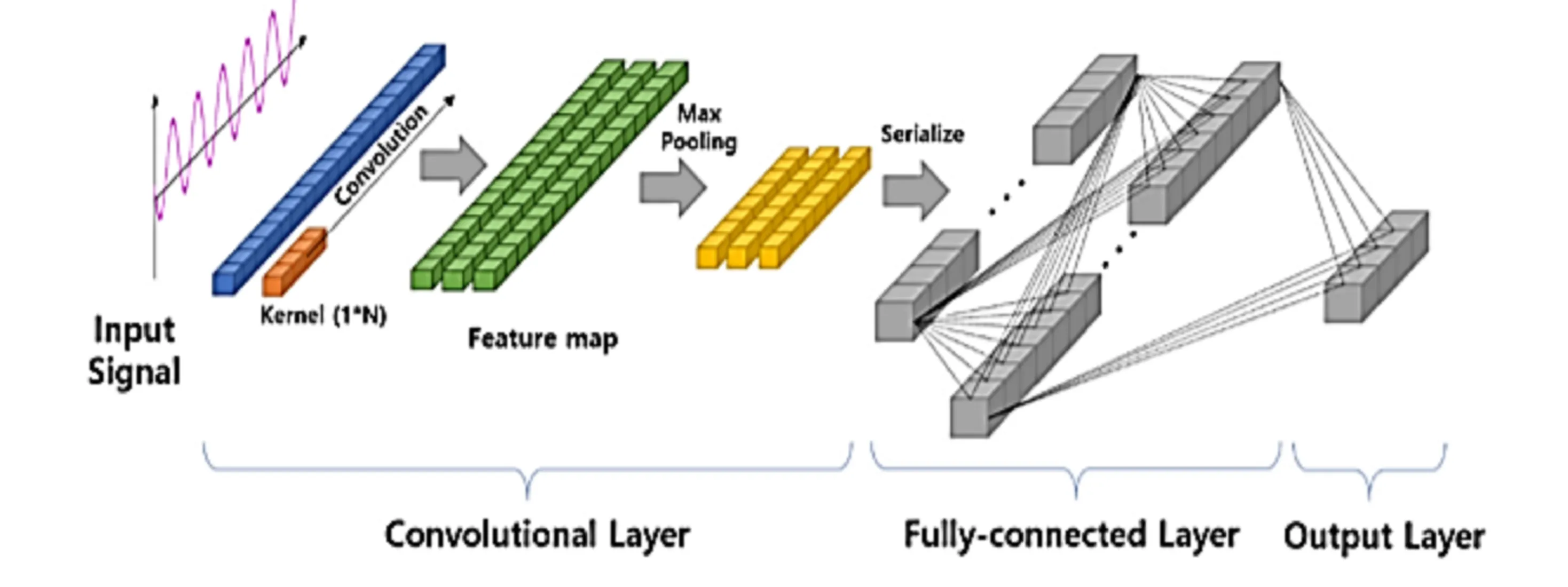
Figure 7 - Visualization of a 1D Convolutional Neural Network

To use this type of network, it seemed preferable to have data in one-hot encoded form (arrays of 0s with only a single 1 at the position of the corresponding letter). Thus we implemented the following function:

def one_hot_encoding(dic):
    tab = []
    erreur = False
    sequences = [sequ for sequ in dic.values()]
    for i in range(len(sequences)):
        tab_lettres = []
        for lettre in sequences[i]:
            one_hot_tab = [0 for i in range(27)]
            if lettre == "-":
                one_hot_tab[0] = 1
                tab_lettres.append(one_hot_tab)
            elif (ord(lettre) <= 90) &  (ord(lettre) >= 65):
                one_hot_tab[ord(lettre)-64] = 1
                tab_lettres.append(one_hot_tab)
            else:
                print("Sequence",i,"has a non-standard value")
                erreur = True
        if not erreur:
            tab.append(tab_lettres)
            erreur = False
    return np.array(tab)

And here is our architecture:

model = Sequential()

model.add(Conv1D(filters=32, kernel_size=5, activation='relu', input_shape=(546,27)))
model.add(MaxPooling1D(pool_size=2))
model.add(Conv1D(filters=64, kernel_size=5, activation='relu'))
model.add(MaxPooling1D(pool_size=2))
model.add(Conv1D(filters=128, kernel_size=3, activation='relu'))
model.add(MaxPooling1D(pool_size=2))
model.add(Conv1D(filters=256, kernel_size=2, activation='relu'))
model.add(MaxPooling1D(pool_size=2))

model.add(Flatten())
model.add(Dense(128,activation='relu'))
model.add(Dropout(0.2))
model.add(Dense(80,activation='relu'))
model.add(Dense(64,activation='relu'))
model.add(Dropout(0.2))
model.add(Dense(32,activation='relu'))
model.add(Dense(18))

To verify and validate proper model functioning, we started by intentionally training it on only 20 sequences (the same for train and test):

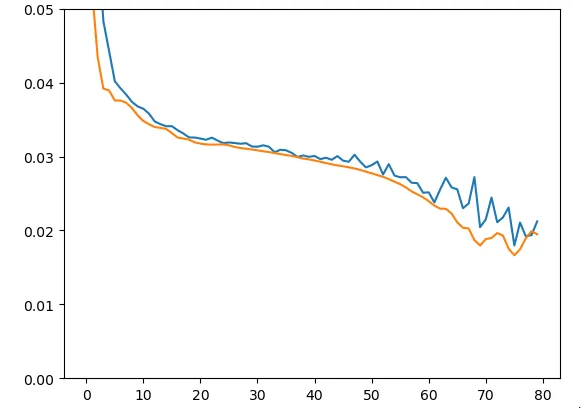
Figure 8 - Train & Test Loss on Training Data

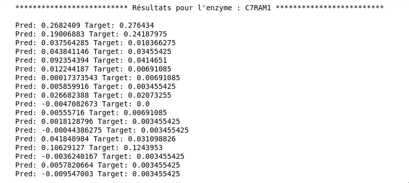
Figure 9 - Results for the Third Model

But what really interests us here is performance on the entire dataset and particularly on a test dataset. Unfortunately, results at this level are not very convincing:

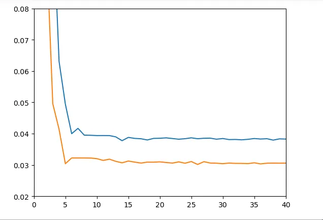
Figure 10 - Train & Test Loss on Dataset

d) Fourth Model: 1D Convolutional Network + LSTM

LSTMs (Long Short Term Memory) form a recurrent neural network (RNN) architecture, capable of acquiring long-term and short-term memory. This is interesting in our case study because given how enzyme active sites work, it is desirable to be able to retain information encoded at the beginning of the sequence to study potential links with amino acids at the other end, for example.

Here is the architecture used:

model = Sequential()
model.add(Conv1D(filters=32, kernel_size=10, activation='relu', input_shape=(546,27)))
model.add(Conv1D(filters=64, kernel_size=7, activation='relu'))
model.add(MaxPooling1D(pool_size=2))
model.add(LSTM(64, return_sequences=True, activation='relu'))
model.add(LSTM(64, return_sequences=True, activation='relu'))

model.add(Conv1D(filters=84, kernel_size=5, activation='relu'))
model.add(Conv1D(filters=128, kernel_size=5, activation='relu'))
model.add(MaxPooling1D(pool_size=2))
model.add(Conv1D(filters=256, kernel_size=3, activation='relu'))
model.add(MaxPooling1D(pool_size=2))
model.add(LSTM(64, return_sequences=True, activation='relu'))
model.add(LSTM(64, return_sequences=True, activation='relu'))

model.add(Flatten())
model.add(Dense(200,activation='relu'))
model.add(Dropout(0.15))
model.add(Dense(100,activation='relu'))
model.add(Dropout(0.15))
model.add(Dense(50,activation='relu'))
model.add(Dense(18))

We obtain results relatively similar to the previous network

Unfortunately, we didn’t have much time to dig into LSTMs. Thus our use of LSTMs in this architecture is probably not very optimal.