MCP Data Science

1. The MCP Protocol

The Model Context Protocol (MCP) is an open-source protocol published by Anthropic in November 2024 to standardize how LLMs interact with external tools and data sources. It relies on JSON-RPC 2.0 and uses stdio as transport: the client starts the server process and communicates with it through standard streams, with no network port or remote service required.

An MCP server can expose three primitives: Tools (callable functions with typed arguments), Resources (read-only consultable data) and Prompts (conversation templates). This project uses exclusively Tools and the instructions field, a text injected into the LLM’s system context upon connection.

The lifecycle of a call is as follows: the LLM decides to call a tool, sends a JSON-RPC message via stdio, the server executes the corresponding Python function and returns a TextContent or ImageContent. The entirety of the reasoning (which tool, in what order, with what arguments) stays in the LLM — the server has no orchestration logic of its own.

FastMCP is the official high-level Python library for MCP. It provides a @mcp.tool() decorator that introspects the Python signature to automatically generate the tool’s JSON Schema, and supports Image returns (binary PNG) in addition to text.

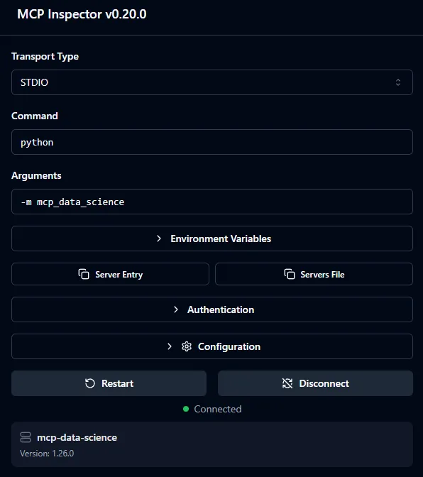
Figure 1 - A tool and its parameters in MCP Inspector

2. Architecture

The server is a single Python process with no external service. It starts in a few seconds with python -m mcp_data_science and immediately exposes its 102 tools.

The server.py file is intentionally minimal (44 lines): it instantiates a single FastMCP object and a single DataStore, then delegates tool registration to each module. This guarantees that all tools share the same state while remaining organized in independent modules.

mcp = FastMCP("mcp-data-science", instructions=_instructions)
store = DataStore()

loading.register_tools(mcp, store)
inspection.register_tools(mcp, store)
# ... 13 other modules

The DataStore

Each MCP call is stateless at the protocol level, but a data science pipeline is inherently stateful: tools pass DataFrames and models from one step to the next. The solution is a singleton DataStore object, instantiated once at startup and passed by reference to each module.

class DataStore:
    _frames : dict[str, pd.DataFrame]  # named DataFrames
    _current: str                       # "active" DataFrame
    _models : dict[str, dict]           # trained ML models
    _plots  : dict[str, bytes]          # PNG plots for reports
    _csv_dir: str                       # output directory

Each tool accepts a df_name: str = "" parameter. If empty, the tool operates on the current DataFrame, allowing the LLM to work without repeating the dataset name at each call, while still supporting multi-dataset scenarios.

3. The 15 Modules and 102 Tools

Module	Tools	Key tools
loading	11	load_csv, load_excel, load_parquet, merge_dataframes, pivot_table
inspection	9	get_head, get_info, quality_report, detect_outliers, get_column_profile
cleaning	9	drop_duplicates, fill_missing, drop_columns, clip_outliers, bin_column
transformation	9	create_column, log_transform, normalize, string_clean, polynomial_features
encoding	4	one_hot_encode, target_encode, label_encode, frequency_encode
visualization	14	plot_histogram, plot_scatter, plot_correlation_matrix, plot_violin, plot_qq
analysis	8	get_correlation, group_aggregate, crosstab, detect_outliers
modeling	8	train_test_split, train_model, evaluate_model, cross_validate, grid_search
feature_selection	4	variance_filter, correlation_filter, feature_importance, drop_low_importance
datetime_tools	4	extract_datetime_parts, datetime_diff, datetime_filter, set_datetime_index
statistical_tests	6	ttest_independent, anova_test, chi_square_test, normality_test, mann_whitney_test
interpretation	7	plot_feature_importance_model, plot_residuals, plot_confusion_matrix, plot_roc_curve
clustering	5	kmeans_cluster, dbscan_cluster, elbow_plot, silhouette_score, cluster_profile
dimensionality	2	pca_transform, tsne_plot
reporting	2	save_report (Markdown + PNGs), save_report_html (self-contained HTML)

Every module follows the same interface contract: tools never raise exceptions (they always return a string, either a success summary or a readable error), docstrings are LLM-facing (FastMCP exposes them directly in the JSON schema), and mutations always go through store.set().

4. The 13-Phase Pipeline

MCP allows a server to inject text into the LLM’s system context upon connection via the instructions field. This project embeds a complete workflow guide (~260 lines) directly in the server. The LLM automatically receives a pipeline structured in 13 phases, decision trees for methodological choices, 12 documented pitfalls to avoid, and an error recovery guide — with no client-side configuration required.

Phase  1 — Loading & First Look       load_csv → get_shape → get_head → get_info
Phase  2 — Exploratory Data Analysis  quality_report → get_statistics → plot_histogram
Phase  3 — Statistical Testing        normality_test → ttest / anova / chi_square
Phase  4 — Data Cleaning              drop_duplicates → fill_missing → clip_outliers
Phase  5 — Feature Engineering        create_column → extract_datetime_parts → log_transform
Phase  6 — Categorical Encoding       one_hot_encode / target_encode / label_encode
Phase  7 — Feature Selection          variance_filter → correlation_filter → feature_importance
Phase  8 — Dimensionality Reduction   pca_transform / tsne_plot
Phase  9 — Normalization              normalize (only for linear/distance-based models)
Phase 10 — Modeling                   train_test_split → train_model → evaluate_model
Phase 11 — Model Interpretation       plot_feature_importance_model → plot_residuals
Phase 12 — Clustering                 elbow_plot → kmeans_cluster → silhouette_score
Phase 13 — Reporting                  save_report / save_report_html

The guide also embeds decision trees for ambiguous choices: which strategy for missing values based on their rate, which statistical test based on the distribution, which categorical encoding based on cardinality. These rules allow the agent to operate rigorously without human intervention.

5. Visualization and Reporting

MCP natively supports binary returns (ImageContent) in addition to text. For data science, this is essential: a correlation heatmap or a QQ-plot cannot be communicated through text. All visualization tools use matplotlib’s Agg backend (headless rendering, no graphical interface) and return an Image object directly via io.BytesIO, with no disk write.

A fig_to_image_and_store() variant also stores the PNG bytes in DataStore._plots to reuse them in the final report without regenerating them.

save_report_html produces a single HTML file with plots embedded as base64, no external dependencies, ready to share. The output follows an 8-section structure (Executive Summary, Data Overview, Exploratory Analysis, Statistical Tests, Cleaning Log, Feature Engineering, Modeling Results, Conclusions) with a complete design system (CSS custom properties, typography, 900px responsive).

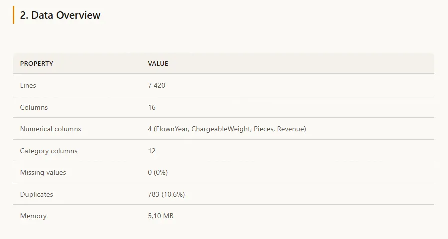
Figure 2 - Data overview in the generated HTML report

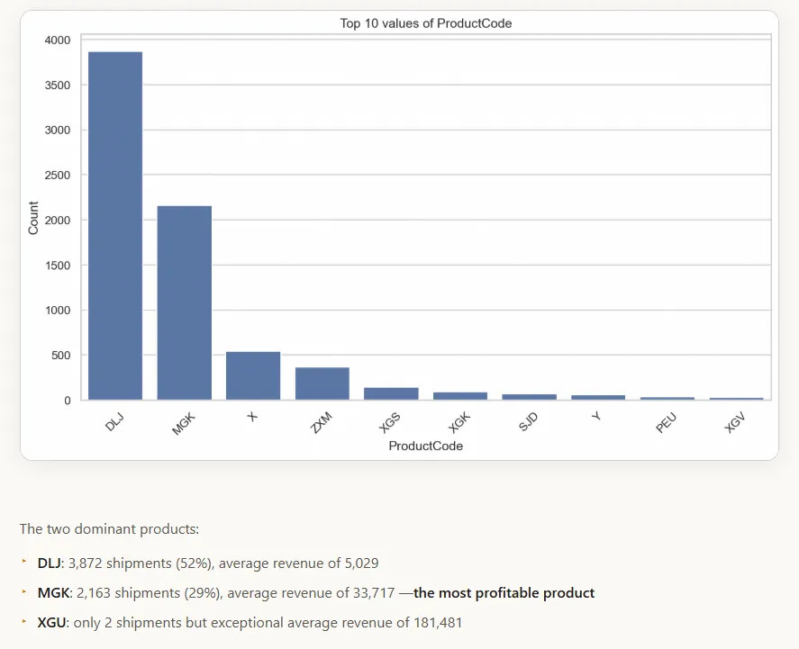
Figure 3 - Generated chart and associated analysis in the HTML report

6. Usage Example

The user asks in natural language: “Load sales_2024.csv, run a quality report, clean the data, train a Random Forest to predict revenue and generate an HTML report.” Claude then orchestrates around twenty tool calls in the correct order, guided by the 13-phase guide embedded in the server.

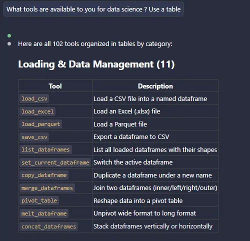
Figure 4 - Usage within Claude Code